Handling Spatial Projection & CRS

Overview

Questions

• What do I do when vector data don’t line up?

Objectives

• Plot vector objects with different CRSs in the same plot.

Prerequisite

Things You’ll Need To Complete This Episode

See the lesson homepage for detailed information about the software, data, and other prerequisites you will need to work through the examples in this episode.

In an earlier episode we learned how to handle a situation where you have two different files with raster data in different projections. Now we will apply those same principles to working with vector data. We will create a base map of our study site using United States state and country boundary information accessed from the United States Census Bureau. We will learn how to map vector data that are in different CRSs and thus don’t line up on a map.

We will continue to work with the three ESRI shapefiles that we loaded in the Open and Plot Vector Layers in R episode.

Working With Spatial Data From Different Sources

---

We often need to gather spatial datasets from different sources and/or data that cover different spatial extents. These data are often in different Coordinate Reference Systems (CRSs).

Some reasons for data being in different CRSs include:

1. The data are stored in a particular CRS convention used by the data provider (for example, a government agency).
2. The data are stored in a particular CRS that is customized to a region. For instance, many states in the US prefer to use a State Plane projection customized for that state.

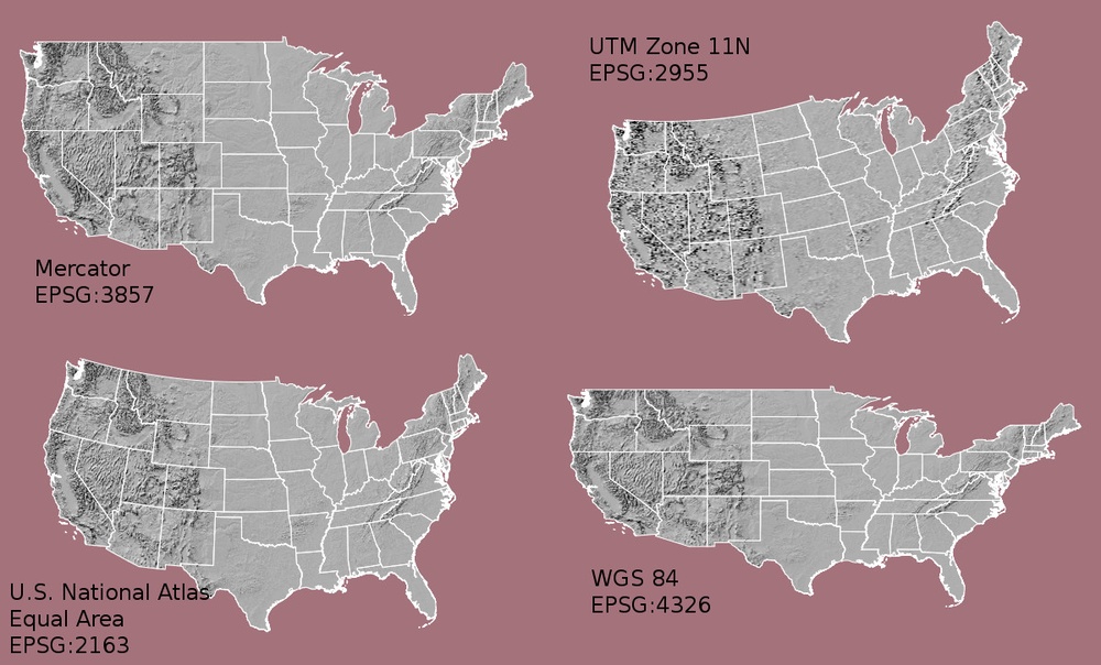{alt=’Maps of the United States using data in different projections.}

Notice the differences in shape associated with each different projection. These differences are a direct result of the calculations used to “flatten” the data onto a 2-dimensional map. Often data are stored purposefully in a particular projection that optimizes the relative shape and size of surrounding geographic boundaries (states, counties, countries, etc).

In this episode we will learn how to identify and manage spatial data in different projections. We will learn how to reproject the data so that they are in the same projection to support plotting / mapping. Note that these skills are also required for any geoprocessing / spatial analysis. Data need to be in the same CRS to ensure accurate results.

We will continue to use the sf and terra packages in this episode.

Import US Boundaries - Census Data

---

There are many good sources of boundary base layers that we can use to create a basemap. Some R packages even have these base layers built in to support quick and efficient mapping. In this episode, we will use boundary layers for the contiguous United States, provided by the United States Census Bureau. It is useful to have vector layers in ESRI’s shapefile format to work with because we can add additional attributes to them if need be - for project specific mapping.

Read US Boundary File

---

We will use the vect() function to import the /US-Boundary-Layers/US-State-Boundaries-Census-2014 layer into R. This layer contains the boundaries of all contiguous states in the U.S. Please note that these data have been modified and reprojected from the original data downloaded from the Census website to support the learning goals of this episode.

R

state_boundary_us <- vect("data/NEON-DS-Site-Layout-Files/US-Boundary-Layers/US-State-Boundaries-Census-2014.shp")

WARNING

Warning: [vect] Z coordinates ignored

Next, let’s plot the U.S. states data:

R

ggplot() +
  geom_spatvector(data = state_boundary_us) +
  ggtitle("Map of Contiguous US State Boundaries") +
  coord_sf()

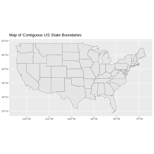
U.S. Boundary Layer

---

We can add a boundary layer of the United States to our map - to make it look nicer. We will import NEON-DS-Site-Layout-Files/US-Boundary-Layers/US-Boundary-Dissolved-States.

R

us_outline <- vect("data/NEON-DS-Site-Layout-Files/US-Boundary-Layers/US-Boundary-Dissolved-States.shp")

WARNING

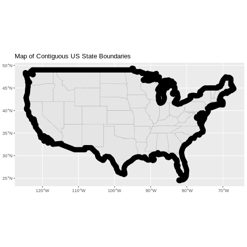
Warning: [vect] Z coordinates ignored

If we specify a thicker line width using size = 2 for the border layer, it will make our map pop! We will also manually set the colors of the state boundaries and country boundaries.

R

ggplot() +
  geom_spatvector(data = state_boundary_us, color = "gray60") +
  geom_spatvector(data = us_outline, color = "black",alpha = 0.25,size = 5) +
  ggtitle("Map of Contiguous US State Boundaries") +
  coord_sf()

Next, let’s add the location of a flux tower where our study area is. As we are adding these layers, take note of the CRS of each object. First let’s look at the CRS of our tower location object:

R

crs(point_harv)

OUTPUT

[1] "PROJCRS[\"WGS 84 / UTM zone 18N\",\n    BASEGEOGCRS[\"WGS 84\",\n        DATUM[\"World Geodetic System 1984\",\n            ELLIPSOID[\"WGS 84\",6378137,298.257223563,\n                LENGTHUNIT[\"metre\",1]]],\n        PRIMEM[\"Greenwich\",0,\n            ANGLEUNIT[\"degree\",0.0174532925199433]],\n        ID[\"EPSG\",4326]],\n    CONVERSION[\"UTM zone 18N\",\n        METHOD[\"Transverse Mercator\",\n            ID[\"EPSG\",9807]],\n        PARAMETER[\"Latitude of natural origin\",0,\n            ANGLEUNIT[\"Degree\",0.0174532925199433],\n            ID[\"EPSG\",8801]],\n        PARAMETER[\"Longitude of natural origin\",-75,\n            ANGLEUNIT[\"Degree\",0.0174532925199433],\n            ID[\"EPSG\",8802]],\n        PARAMETER[\"Scale factor at natural origin\",0.9996,\n            SCALEUNIT[\"unity\",1],\n            ID[\"EPSG\",8805]],\n        PARAMETER[\"False easting\",500000,\n            LENGTHUNIT[\"metre\",1],\n            ID[\"EPSG\",8806]],\n        PARAMETER[\"False northing\",0,\n            LENGTHUNIT[\"metre\",1],\n            ID[\"EPSG\",8807]]],\n    CS[Cartesian,2],\n        AXIS[\"(E)\",east,\n            ORDER[1],\n            LENGTHUNIT[\"metre\",1]],\n        AXIS[\"(N)\",north,\n            ORDER[2],\n            LENGTHUNIT[\"metre\",1]],\n    ID[\"EPSG\",32618]]"

Our project string for point_harv specifies the UTM projection as follows:

+proj=utm +zone=18 +datum=WGS84 +units=m +no_defs

• proj=utm: the projection is UTM, UTM has several zones.
• zone=18: the zone is 18
• datum=WGS84: the datum WGS84 (the datum refers to the 0,0 reference for the coordinate system used in the projection)
• units=m: the units for the coordinates are in METERS.

Note that the zone is unique to the UTM projection. Not all CRSs will have a zone.

Let’s check the CRS of our state and country boundary objects:

R

crs(state_boundary_us)

OUTPUT

[1] "GEOGCRS[\"WGS 84\",\n    DATUM[\"World Geodetic System 1984\",\n        ELLIPSOID[\"WGS 84\",6378137,298.257223563,\n            LENGTHUNIT[\"metre\",1]]],\n    PRIMEM[\"Greenwich\",0,\n        ANGLEUNIT[\"degree\",0.0174532925199433]],\n    CS[ellipsoidal,2],\n        AXIS[\"geodetic latitude (Lat)\",north,\n            ORDER[1],\n            ANGLEUNIT[\"degree\",0.0174532925199433]],\n        AXIS[\"geodetic longitude (Lon)\",east,\n            ORDER[2],\n            ANGLEUNIT[\"degree\",0.0174532925199433]],\n    ID[\"EPSG\",4326]]"

R

crs(us_outline)

OUTPUT

[1] "GEOGCRS[\"WGS 84\",\n    DATUM[\"World Geodetic System 1984\",\n        ELLIPSOID[\"WGS 84\",6378137,298.257223563,\n            LENGTHUNIT[\"metre\",1]]],\n    PRIMEM[\"Greenwich\",0,\n        ANGLEUNIT[\"degree\",0.0174532925199433]],\n    CS[ellipsoidal,2],\n        AXIS[\"geodetic latitude (Lat)\",north,\n            ORDER[1],\n            ANGLEUNIT[\"degree\",0.0174532925199433]],\n        AXIS[\"geodetic longitude (Lon)\",east,\n            ORDER[2],\n            ANGLEUNIT[\"degree\",0.0174532925199433]],\n    ID[\"EPSG\",4326]]"

Our project string for state_boundary_us and us_outline specifies the lat/long projection as follows:

+proj=longlat +datum=WGS84 +no_defs

• proj=longlat: the data are in a geographic (latitude and longitude) coordinate system
• datum=WGS84: the datum WGS84 (the datum refers to the 0,0 reference for the coordinate system used in the projection)
• no_defs: ensures that no defaults are used, but this is now obsolete

Note that there are no specified units above. This is because this geographic coordinate reference system is in latitude and longitude which is most often recorded in decimal degrees.

Callout

Data Tip

the last portion of each proj4 string could potentially be something like +towgs84=0,0,0. This is a conversion factor that is used if a datum conversion is required. We will not deal with datums in this episode series.

CRS Units - View Object Extent

---

Next, let’s view the extent or spatial coverage for the point_harv spatial object compared to the state_boundary_us object.

First we’ll look at the extent for our study site:

R

ext(point_harv)

OUTPUT

SpatExtent : 732183.193775523, 732183.193775523, 4713265.04113709, 4713265.04113709 (xmin, xmax, ymin, ymax)

And then the extent for the state boundary data.

R

ext(state_boundary_us)

OUTPUT

SpatExtent : -124.725839, -66.949895, 24.498131, 49.384358 (xmin, xmax, ymin, ymax)

Note the difference in the units for each object. The extent for state_boundary_us is in latitude and longitude which yields smaller numbers representing decimal degree units. Our tower location point is in UTM, is represented in meters.

Callout

Proj4 & CRS Resources

• Official PROJ library documentation
• More information on the proj4 format.
• A fairly comprehensive list of CRSs by format.
• To view a list of datum conversion factors type: sf_proj_info(type = "datum") into the R console. However, the results would depend on the underlying version of the PROJ library.

Reproject Vector Data or No?

---

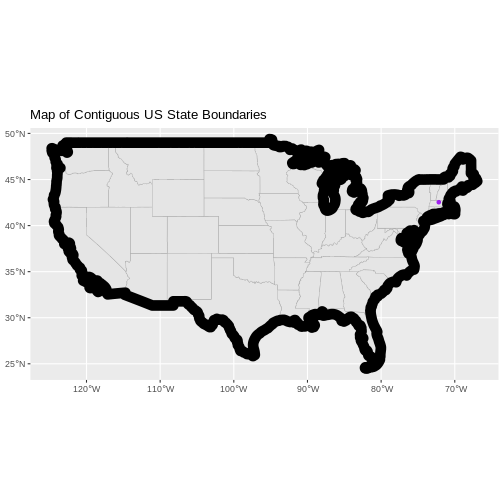
We saw in an earlier episode that when working with raster data in different CRSs, we needed to convert all objects to the same CRS. We can do the same thing with our vector data - however, we don’t need to! When using the ggplot2 package, ggplot automatically converts all objects to the same CRS before plotting. This means we can plot our three data sets together without doing any conversion:

R

ggplot() +
  geom_spatvector(data = state_boundary_us, color = "gray60") +
  geom_spatvector(data = us_outline, size = 5, alpha = 0.25, color = "black") +
  geom_spatvector(data = point_harv, shape = 19, color = "purple") +
  ggtitle("Map of Contiguous US State Boundaries") +
  coord_sf()

Challenge

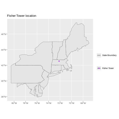
Challenge - Plot Multiple Layers of Spatial Data

Create a map of the North Eastern United States as follows:

1. Import and plot Boundary-US-State-NEast.shp. Adjust line width as necessary.
2. Layer the Fisher Tower (in the NEON Harvard Forest site) point location point_harv onto the plot.
3. Add a title.
4. Add a legend that shows both the state boundary (as a line) and the Tower location point.

Answers

R

ne_states_outline <- vect("data/NEON-DS-Site-Layout-Files/US-Boundary-Layers/Boundary-US-State-NEast.shp")

WARNING

Warning: [vect] Z coordinates ignored

R

ggplot() +
    geom_spatvector(data = ne_states_outline, aes(color ="color"),
            show.legend = "line") +
    scale_color_manual(name = "", labels = "State Boundary",
                       values = c("color" = "gray18")) +
    geom_spatvector(data = point_harv, aes(shape = "shape"), color = "purple") +
    scale_shape_manual(name = "", labels = "Fisher Tower",
                       values = c("shape" = 19)) +
    ggtitle("Fisher Tower location") +
    theme(legend.background = element_rect(color = NA)) +
    coord_sf()

Key Points

• ggplot2 automatically converts all objects in a plot to the same CRS.
• Still be aware of the CRS and extent for each object.