Open and Plot Vector Layers
Last updated on 2026-02-05 | Edit this page
Overview
Questions
- How can I distinguish between and visualize point, line and polygon vector data?
Objectives
- Know the difference between point, line, and polygon vector elements.
- Load point, line, and polygon vector layers into R.
- Access the attributes of a spatial object in R.
Things You’ll Need To Complete This Episode
See the lesson homepage for detailed information about the software, data, and other prerequisites you will need to work through the examples in this episode.
This lesson begins with vector data - points, lines, and polygons that represent discrete geographic features. Vector data is often familiar to researchers who work with field observations or survey data. After mastering vector data in Episodes 01-05, we’ll move to raster data (Episodes 06-10), which represents continuous surfaces using grids of pixels.
In this episode, we will open and plot point, line and polygon vector
data loaded from ESRI’s shapefile format into R. These data
refer to the NEON
Harvard Forest field site. In later episodes, we will learn how to
work with raster and vector data together and combine them into a single
plot.
Import Vector Data
We will use the terra package to work with both vector
and raster data in R. Using a single package for both data types
simplifies our workflow and provides consistent syntax across geospatial
operations. The tidyterra package extends
terra with tidyverse-style functions and ggplot2
integration.
Why terra?
The terra package is the modern successor to the
raster package, offering significant advantages:
- Performance: Much faster processing, especially for large datasets
- Memory efficiency: Better handling of data that doesn’t fit in RAM
- Unified interface: Consistent functions for both vector (SpatVector) and raster (SpatRaster) data
- Active development: Actively maintained with regular updates and improvements
-
Integration: Works seamlessly with tidyverse
through the
tidyterrapackage
While you may encounter the sf package in older
tutorials (which remains excellent for vector-only workflows),
terra represents the current best practice for geospatial
analysis in R, especially when working with both vector and raster
data.
Make sure you have the terra and tidyterra
libraries loaded.
R
library(terra)
library(tidyterra)
The vector layers that we will import from ESRI’s
shapefile format are:
- A polygon vector layer representing our field site boundary,
- A line vector layer representing roads, and
- A point vector layer representing the location of the Fisher flux tower located at the NEON Harvard Forest field site.
The first vector layer that we will open contains the boundary of our
study area (or our Area Of Interest or AOI, hence the name
aoiBoundary). To import a vector layer from an ESRI
shapefile we use the terra function
vect(). vect() requires the file path to the
ESRI shapefile.
Let’s import our AOI:
R
aoi_boundary_harv <- vect(
  "data/NEON-DS-Site-Layout-Files/HARV/HarClip_UTMZ18.shp")
Vector Layer Metadata & Attributes
When we import the HarClip_UTMZ18 vector layer from an
ESRI shapefile into R (as our
aoi_boundary_harv object), the vect() function
automatically stores information about the data. We are particularly
interested in the geospatial metadata, describing the format, CRS,
extent, and other components of the vector data, and the attributes
which describe properties associated with each individual vector
object.
Data Tip
The Explore and Plot by Vector Layer Attributes episode provides more information on both metadata and attributes and using attributes to subset and plot data.
Spatial Metadata
Key metadata for all vector layers includes:
- Object Type: the class of the imported object.
- Coordinate Reference System (CRS): the projection of the data.
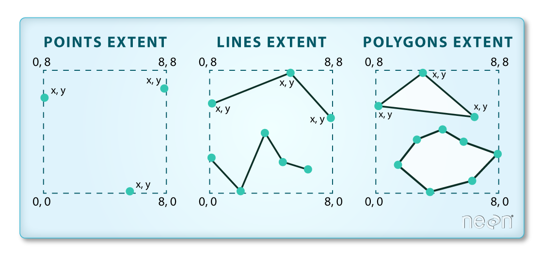
- Extent: the spatial extent (i.e. geographic area that the vector layer covers) of the data. Note that the spatial extent for a vector layer represents the combined extent for all individual objects in the vector layer.
We can view metadata of a vector layer using the
geomtype(), crs() and ext()
functions. First, let’s view the geometry type for our AOI vector
layer:
R
geomtype(aoi_boundary_harv)
OUTPUT
[1] "polygons"Our aoi_boundary_harv is a polygon spatial object. Now
let’s check what CRS this file data is in:
R
crs(aoi_boundary_harv)
OUTPUT
[1] "PROJCRS[\"WGS 84 / UTM zone 18N\",\n BASEGEOGCRS[\"WGS 84\",\n DATUM[\"World Geodetic System 1984\",\n ELLIPSOID[\"WGS 84\",6378137,298.257223563,\n LENGTHUNIT[\"metre\",1]]],\n PRIMEM[\"Greenwich\",0,\n ANGLEUNIT[\"degree\",0.0174532925199433]],\n ID[\"EPSG\",4326]],\n CONVERSION[\"UTM zone 18N\",\n METHOD[\"Transverse Mercator\",\n ID[\"EPSG\",9807]],\n PARAMETER[\"Latitude of natural origin\",0,\n ANGLEUNIT[\"Degree\",0.0174532925199433],\n ID[\"EPSG\",8801]],\n PARAMETER[\"Longitude of natural origin\",-75,\n ANGLEUNIT[\"Degree\",0.0174532925199433],\n ID[\"EPSG\",8802]],\n PARAMETER[\"Scale factor at natural origin\",0.9996,\n SCALEUNIT[\"unity\",1],\n ID[\"EPSG\",8805]],\n PARAMETER[\"False easting\",500000,\n LENGTHUNIT[\"metre\",1],\n ID[\"EPSG\",8806]],\n PARAMETER[\"False northing\",0,\n LENGTHUNIT[\"metre\",1],\n ID[\"EPSG\",8807]]],\n CS[Cartesian,2],\n AXIS[\"(E)\",east,\n ORDER[1],\n LENGTHUNIT[\"metre\",1]],\n AXIS[\"(N)\",north,\n ORDER[2],\n LENGTHUNIT[\"metre\",1]],\n ID[\"EPSG\",32618]]"Our data in the CRS UTM zone 18N. The CRS is
critical to interpreting the spatial object’s extent values as it
specifies units. To find the extent of our AOI, we can use the
ext() function:
R
ext(aoi_boundary_harv)
OUTPUT
SpatExtent : 732128.016925, 732251.102892, 4713208.71096, 4713359.17112 (xmin, xmax, ymin, ymax)The spatial extent of a vector layer or R spatial object represents the geographic “edge” or location that is the furthest north, south east and west. Thus it represents the overall geographic coverage of the spatial object. Image Source: National Ecological Observatory Network (NEON).
Lastly, we can view all of the metadata and attributes for this R spatial object by printing it to the screen:
R
aoi_boundary_harv
OUTPUT
 class       : SpatVector
 geometry    : polygons
 dimensions  : 1, 1  (geometries, attributes)
 extent      : 732128, 732251.1, 4713209, 4713359  (xmin, xmax, ymin, ymax)
 source      : HarClip_UTMZ18.shp
 coord. ref. : WGS 84 / UTM zone 18N (EPSG:32618)
 names       :    id
 type        : <num>
 values      :     1
Spatial Data Attributes
We introduced the idea of spatial data attributes in an earlier lesson. Now we will explore how to use spatial data attributes stored in our data to plot different features.
Plot a vector layer
Next, let’s visualize the data in our SpatVector object
using the ggplot package. Unlike with raster data, we do
not need to convert vector data to a dataframe before plotting with
ggplot.
We’re going to customize our boundary plot by setting the size,
color, and fill for our plot. When plotting SpatVector
objects with ggplot2, we use geom_spatvector()
from the tidyterra package, which requires the
coord_sf() coordinate system.
R
ggplot() +
  geom_spatvector(data = aoi_boundary_harv, size = 3, color = "black", fill = "cyan1") +
  ggtitle("AOI Boundary Plot") +
  coord_sf()
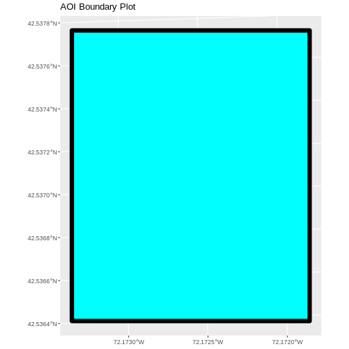
On what may be the most boring plot ever, the x and y axes are
labeled in units of decimal degrees. However, the CRS for
aoi_boundary_harv is UTM zone 18N, which has units of
meters. geom_spatvector() will use the CRS of the data to
set the CRS for the plot, so why is there a mismatch?
By default, coord_sf() generates a graticule with a CRS
of WGS 84 (where the units are decimal degrees), and this sets our axis
labels. To draw the graticule in the native CRS of our shapefile, we can
set datum=NULL in the coord_sf() function.
Challenge: Import Line and Point Vector Layers
Using the steps above, import the HARV_roads and HARVtower_UTM18N
vector layers into R. Call the HARV_roads object lines_harv
and the HARVtower_UTM18N point_harv.
Answer the following questions:
What type of R spatial object is created when you import each layer?
What is the CRS and extent for each object?
Do the files contain points, lines, or polygons?
How many spatial objects are in each file?
First we import the data:
R
lines_harv <- vect("data/NEON-DS-Site-Layout-Files/HARV/HARV_roads.shp")
point_harv <- vect("data/NEON-DS-Site-Layout-Files/HARV/HARVtower_UTM18N.shp")
Then we check its class:
R
class(lines_harv)
OUTPUT
[1] "SpatVector"
attr(,"package")
[1] "terra"
R
class(point_harv)
OUTPUT
[1] "SpatVector"
attr(,"package")
[1] "terra"
We also check the CRS and extent of each object:
R
crs(lines_harv)
OUTPUT
[1] "PROJCRS[\"WGS 84 / UTM zone 18N\",\n BASEGEOGCRS[\"WGS 84\",\n DATUM[\"World Geodetic System 1984\",\n ELLIPSOID[\"WGS 84\",6378137,298.257223563,\n LENGTHUNIT[\"metre\",1]]],\n PRIMEM[\"Greenwich\",0,\n ANGLEUNIT[\"degree\",0.0174532925199433]],\n ID[\"EPSG\",4326]],\n CONVERSION[\"UTM zone 18N\",\n METHOD[\"Transverse Mercator\",\n ID[\"EPSG\",9807]],\n PARAMETER[\"Latitude of natural origin\",0,\n ANGLEUNIT[\"Degree\",0.0174532925199433],\n ID[\"EPSG\",8801]],\n PARAMETER[\"Longitude of natural origin\",-75,\n ANGLEUNIT[\"Degree\",0.0174532925199433],\n ID[\"EPSG\",8802]],\n PARAMETER[\"Scale factor at natural origin\",0.9996,\n SCALEUNIT[\"unity\",1],\n ID[\"EPSG\",8805]],\n PARAMETER[\"False easting\",500000,\n LENGTHUNIT[\"metre\",1],\n ID[\"EPSG\",8806]],\n PARAMETER[\"False northing\",0,\n LENGTHUNIT[\"metre\",1],\n ID[\"EPSG\",8807]]],\n CS[Cartesian,2],\n AXIS[\"(E)\",east,\n ORDER[1],\n LENGTHUNIT[\"metre\",1]],\n AXIS[\"(N)\",north,\n ORDER[2],\n LENGTHUNIT[\"metre\",1]],\n ID[\"EPSG\",32618]]"R
ext(lines_harv)
OUTPUT
SpatExtent : 730741.189051256, 733295.54863222, 4711942.00505579, 4714259.95719612 (xmin, xmax, ymin, ymax)R
crs(point_harv)
OUTPUT
[1] "PROJCRS[\"WGS 84 / UTM zone 18N\",\n BASEGEOGCRS[\"WGS 84\",\n DATUM[\"World Geodetic System 1984\",\n ELLIPSOID[\"WGS 84\",6378137,298.257223563,\n LENGTHUNIT[\"metre\",1]]],\n PRIMEM[\"Greenwich\",0,\n ANGLEUNIT[\"degree\",0.0174532925199433]],\n ID[\"EPSG\",4326]],\n CONVERSION[\"UTM zone 18N\",\n METHOD[\"Transverse Mercator\",\n ID[\"EPSG\",9807]],\n PARAMETER[\"Latitude of natural origin\",0,\n ANGLEUNIT[\"Degree\",0.0174532925199433],\n ID[\"EPSG\",8801]],\n PARAMETER[\"Longitude of natural origin\",-75,\n ANGLEUNIT[\"Degree\",0.0174532925199433],\n ID[\"EPSG\",8802]],\n PARAMETER[\"Scale factor at natural origin\",0.9996,\n SCALEUNIT[\"unity\",1],\n ID[\"EPSG\",8805]],\n PARAMETER[\"False easting\",500000,\n LENGTHUNIT[\"metre\",1],\n ID[\"EPSG\",8806]],\n PARAMETER[\"False northing\",0,\n LENGTHUNIT[\"metre\",1],\n ID[\"EPSG\",8807]]],\n CS[Cartesian,2],\n AXIS[\"(E)\",east,\n ORDER[1],\n LENGTHUNIT[\"metre\",1]],\n AXIS[\"(N)\",north,\n ORDER[2],\n LENGTHUNIT[\"metre\",1]],\n ID[\"EPSG\",32618]]"R
ext(point_harv)
OUTPUT
SpatExtent : 732183.193775523, 732183.193775523, 4713265.04113709, 4713265.04113709 (xmin, xmax, ymin, ymax)To see the number of objects in each file, we can look at the output
from when we read these objects into R. lines_harv contains
13 features (all lines) and point_harv contains only one
point.
- Metadata for vector layers include geometry type, CRS, and extent.
- Load spatial objects into R with the
vect()function from theterrapackage. - Spatial objects can be plotted directly with
ggplotusing thegeom_spatvector()function fromtidyterra. No need to convert to a dataframe.